Basic workflow

library(HSItools)
#> Warning: replacing previous import 'DT::dataTableOutput' by
#> 'shiny::dataTableOutput' when loading 'HSItools'
#> Warning: replacing previous import 'DT::renderDataTable' by
#> 'shiny::renderDataTable' when loading 'HSItools'
library(patchwork)
library(terra)
#> terra 1.7.78
#> 
#> Attaching package: 'terra'
#> The following object is masked from 'package:patchwork':
#> 
#>     area
library(dplyr)
#> 
#> Attaching package: 'dplyr'
#> The following objects are masked from 'package:terra':
#> 
#>     intersect, union
#> The following objects are masked from 'package:stats':
#> 
#>     filter, lag
#> The following objects are masked from 'package:base':
#> 
#>     intersect, setdiff, setequal, union
library(tidyr)
#> 
#> Attaching package: 'tidyr'
#> The following object is masked from 'package:terra':
#> 
#>     extract
library(ggplot2)

Here, we present a basic workflow for a single core. It is assumed that the output of the run_core() function is available and stored on the disk.

We’re using some internal data here, substantially reducing spatial resolution.

Typically at this point you are going to use the shiny app output of the run_core() function stored in the *.rds file. Here, for the vignette we recreate this output by hand. You can also produce these files this way, without running shiny app.

# Load run_core() output

core <- list(
  analysisOptions = list(
    normalize = TRUE,
    integration = FALSE,
    proxies = 'rabd_b660b670'
  ),
  layers = c(560.84, 585.49, 610.24, 635.08, 660.02, 685.05, 710.19, 735.41),
  cropImage = c(948, 1283, 13143, 13211),
  simpleRGB = list(ext = c(xmin = 88, xmax = 1287, ymin = 13132, ymax = 13217)),
  rasterPaths = list(
    capture = fs::path_package(package = "HSItools", "extdata/CORE_XYZ/CORE_XYZ.tif"),
    darkref = fs::path_package(package = "HSItools", "extdata/CORE_XYZ/DARKREF_CORE_XYZ.tif"),
    whiteref = fs::path_package(package = "HSItools", "extdata/CORE_XYZ/WHITEREF_CORE_XYZ.tif")
  ),
  directory = fs::path_package(package = "HSItools", "extdata/CORE_XYZ"),
  analysisRegions = NULL,
  distances = list(
    startCore = c(x = 1133, y = 13217),
    endCore = c(x = 1133, y = 13132),
    startScale = c(x = 1148, y = 13206),
    endScale = c(x = 1149, y = 13137),
    coreDist = 69,
    scaleDist = 70,
    scaleDistmm = 6,
    pixelRatio = 0.0857142857142857
  )
)

Preprocessing

Normalization

Before any spectral indices and properties are calculated, normalizing the data and expressing it as a reflectance is necessary.

# Here we use run_core() output, so further function arguments are filled automatically.
# Output is written to the file.
reflectance <- core |>
  prepare_core()
#> |---------|---------|---------|---------|=========================================                                          |---------|---------|---------|---------|=========================================                                          |---------|---------|---------|---------|=========================================                                          |---------|---------|---------|---------|=========================================

At this stage, we can plot the RGB preview. Our example file has only eight random wavelengths, so it is impossible to plot true RGB. Instead, we use the first, middle, and last available layer, which results in a somewhat gray image. Additionally, we provide calibration so depths are displayed as mm rather than pixels; don’t mind the odd values.

plot_raster_rgb(
  reflectance,
  calibration = pixel_to_distance(core))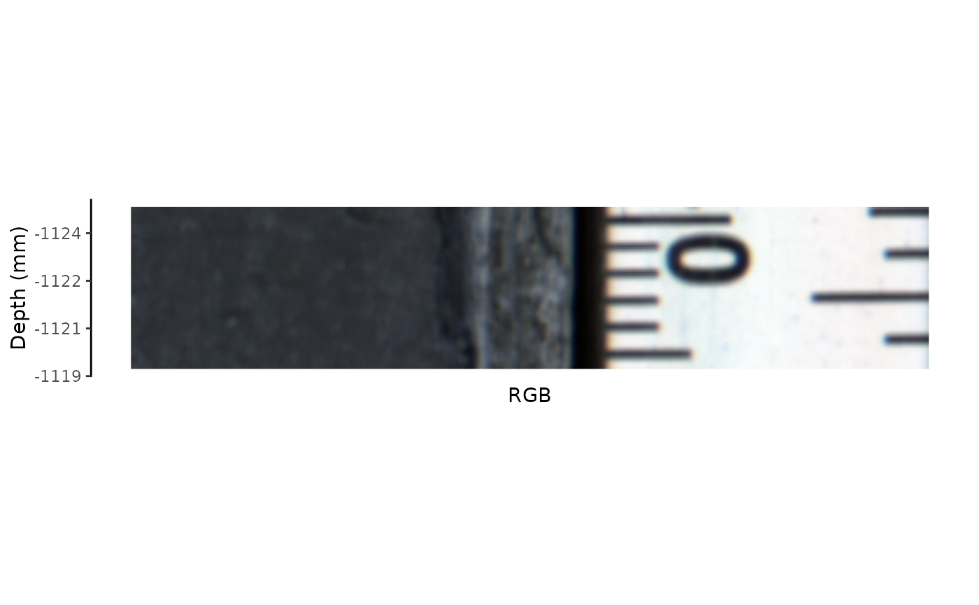

Spectral smoothing

Applying spectral smoothing, such as the Savitzky-Golay spectral filter (Savitzky and Golay 1964), is a good idea. Spurious, random peaks and throughs do not influence the calculation results as much.

reflectance_smooth <- reflectance |>
  # Specify the file extension
  filter_savgol()
#> |---------|---------|---------|---------|=========================================

We can plot the RGB preview at this stage, too.

plot_raster_rgb(
  reflectance_smooth,
  calibration = pixel_to_distance(core))

Peek into spectra

Let’s compare these two spectra. Unsurprisingly, they are very similar again—the number of wavelengths is drastically reduced.

# Spectral profile from the entire ROI
reflectance_sp <- reflectance |>
  # Use HSItools function to extract the profile
  extract_spectral_profile() |>
  # Pivot longer so for plotting
  tidyr::pivot_longer(
    dplyr::everything(),
    names_to = "band",
    values_to = "reflectance",
    names_transform = readr::parse_number)

# Peek into data
head(reflectance_sp)
#> # A tibble: 6 × 2
#>    band reflectance
#>   <dbl>       <dbl>
#> 1  561.       0.297
#> 2  585.       0.303
#> 3  610.       0.297
#> 4  635.       0.298
#> 5  660.       0.292
#> 6  685.       0.276

# Spectral profile from the entire ROI
reflectance_smooth_sp <- reflectance_smooth |>
  # Use HSItools function to extract the profile
  extract_spectral_profile() |>
  # Pivot longer so for plotting
  tidyr::pivot_longer(
    dplyr::everything(),
    names_to = "band",
    values_to = "reflectance_sg",
    names_transform = readr::parse_number)

# Peek into data
head(reflectance_smooth_sp)
#> # A tibble: 6 × 2
#>    band reflectance_sg
#>   <dbl>          <dbl>
#> 1  561.          0.297
#> 2  585.          0.303
#> 3  610.          0.297
#> 4  635.          0.298
#> 5  660.          0.292
#> 6  685.          0.277

# Plot both profiles data
sp_compare <- dplyr::left_join(
  reflectance_sp,
  reflectance_smooth_sp,
  dplyr::join_by(band)) |>
  tidyr::pivot_longer(
    -band,
    names_to = "type",
    values_to = "reflectance") |>
  ggplot2::ggplot(
    aes(
      band,
      reflectance,
      color = type)) +
  ggplot2::geom_line() +
  ggplot2::scale_x_continuous(
    breaks = scales::pretty_breaks()) +
  ggplot2::labs(
    x = "Wavelength (nm)",
    y = "Reflectance",
    color = "Spectrum type") +
  ggplot2::theme_bw() +
  ggplot2::theme(legend.position = "bottom")

# Print
sp_compare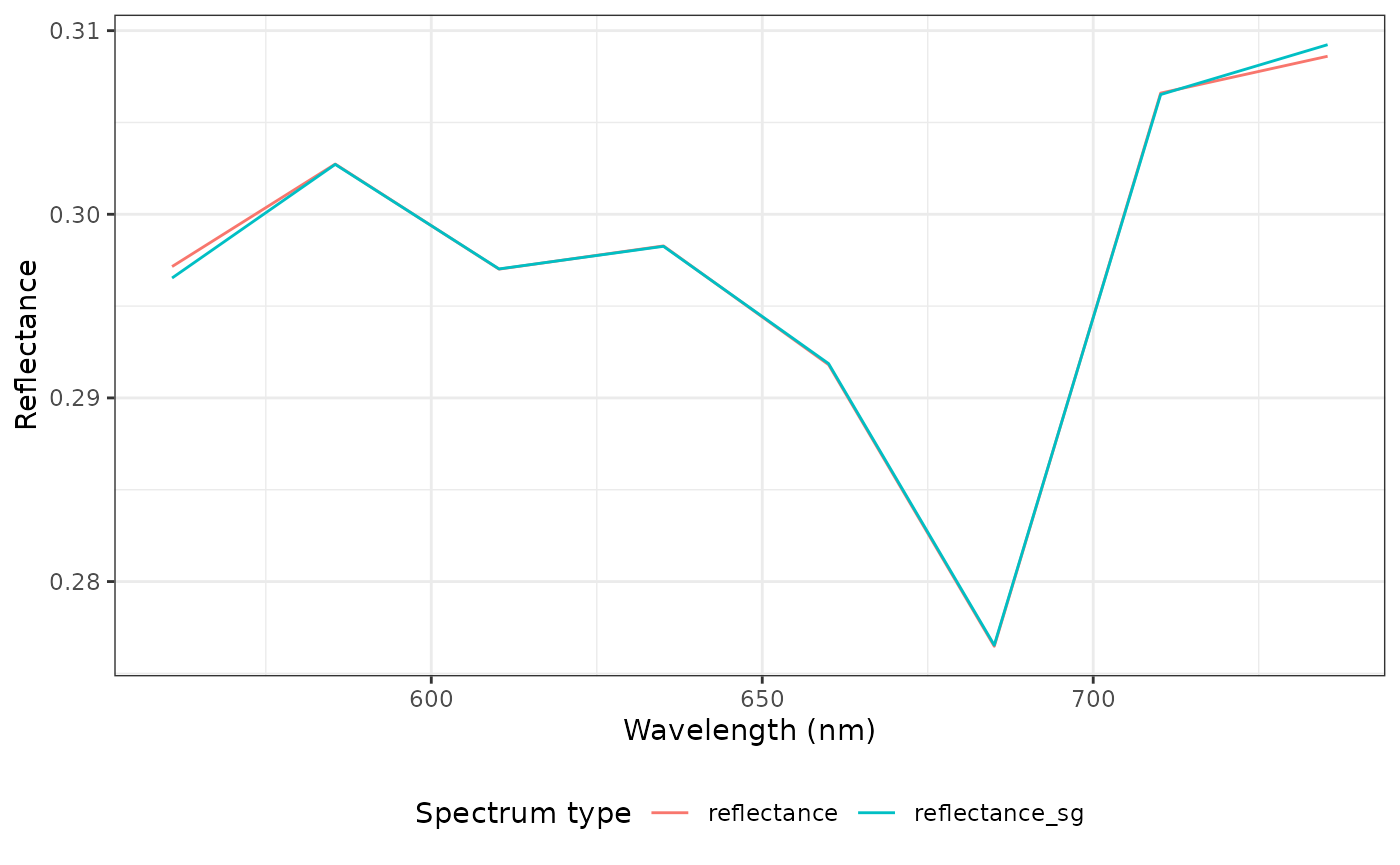

Continuum removal

We can process our data further by removing the continuum, which follows the rule of dividing the spectrum by its bounding box. This way, the spectrum becomes flatter.

# Calculate reflectance with removed continuum
# Use the smoothed spectrum
reflectance_cr <- reflectance_smooth |>
  remove_continuum()
#> |---------|---------|---------|---------|=========================================

Index calculation

At this point, we can start calculating selected indices or proxies.

Mean reflectance (Rmean)

rmean <- reflectance_smooth |>
  calculate_rmean()

plot_rmean <- rmean |>
  plot_raster_proxy(
    hsi_index = names(rmean),
    palette = "mako",
    calibration = pixel_to_distance(core))

# Print
plot_rmean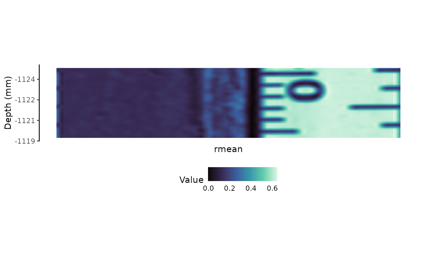

Relative Absorption Band Depth (RABD).

The RABD calculation has variations, but the results are generally not drastically different. Let’s calculate one of the most common indices to estimate the total chloropigments-a: RABD_660:670.

You can use predefined values or provide them manually. Let’s calculate three different flavors.

The name of the output informs you about the calculated proxy and additional modifications to the reflectance file; here, we see that it was calculated with Savitzky-Golay smoothed reflectance.

Variant 1: max

In this variant, a minimum reflectance is found in the trough for each pixel and flexibly used for calculations.

rabd660670max <- reflectance_smooth |>
  # Calculate max variant
  calculate_rabd(
    edges = proxies$rabd_b660b670$edges,
    trough = proxies$rabd_b660b670$trough,
    rabd_name = proxies$rabd_b660b670$proxy_name,
    rabd_type = "max")
#> |---------|---------|---------|---------|=========================================

Plot. Hyperspectral imaging data is most interesting when visualized. We use viridis palettes. There is not much to see, and values are unrealistic because the number of layers is dramatically reduced.

# Prepare the plot
plot_rabd660670max <- rabd660670max |>
  plot_raster_proxy(
    hsi_index = names(rabd660670max),
    palette = "viridis",
    calibration = pixel_to_distance(core))

# Print
plot_rabd660670max

Variant 2: strict

This classic variant supplies a specific wavelength to calculate RABD for every pixel.

rabd665 <- reflectance_smooth |>
  # Calculate max variant
  calculate_rabd(
    edges = proxies$rabd_b660b670$edges,
    trough = 665,
    rabd_name = proxies$rabd_b660b670$proxy_name,
    rabd_type = "strict")
#> |---------|---------|---------|---------|=========================================

# Prepare the plot
plot_rabd665 <- rabd665 |>
  plot_raster_proxy(
    hsi_index = names(rabd665),
    palette = "viridis",
    calibration = pixel_to_distance(core))

# Print
plot_rabd665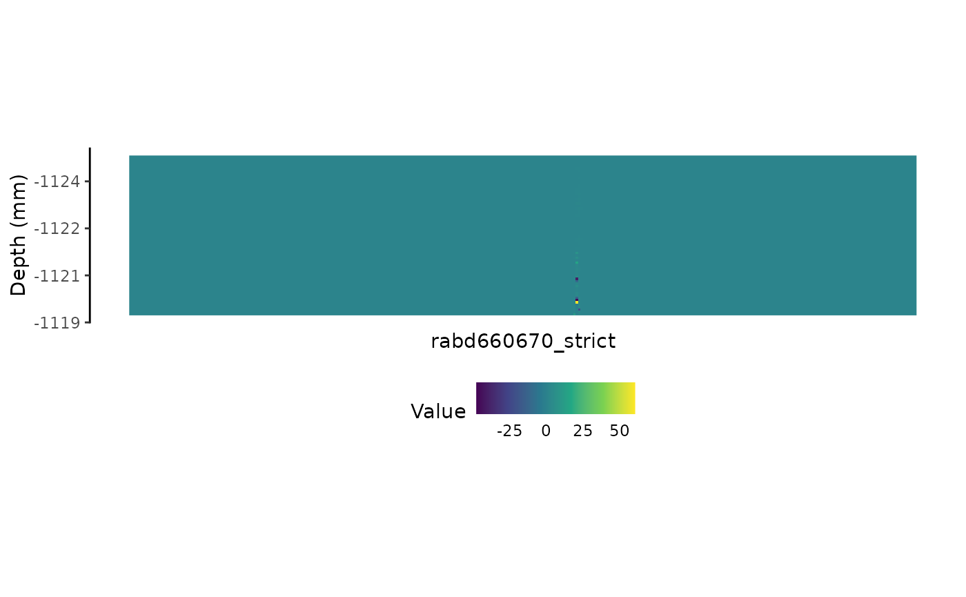

Variant 3: midpoint

This is variant 2 (strict), with the added shortcut of always finding the middle point between the through edges.

rabd660670mid <- reflectance_smooth |>
  # Calculate max variant
  calculate_rabd(
    edges = proxies$rabd_b660b670$edges,
    trough = proxies$rabd_b660b670$trough,
    rabd_name = proxies$rabd_b660b670$proxy_name,
    rabd_type = "mid")
#> |---------|---------|---------|---------|=========================================

# Prepare the plot
plot_rabd660670mid <- rabd660670mid |>
  plot_raster_proxy(
    hsi_index = names(rabd660670mid),
    palette = "viridis",
    calibration = pixel_to_distance(core))

# Print
plot_rabd660670mid

Compare

We can compare these three plots side by side. We’re using patchwork.

plot_rabd660670max + plot_rabd665 + plot_rabd660670mid + patchwork::plot_layout(nrow = 1)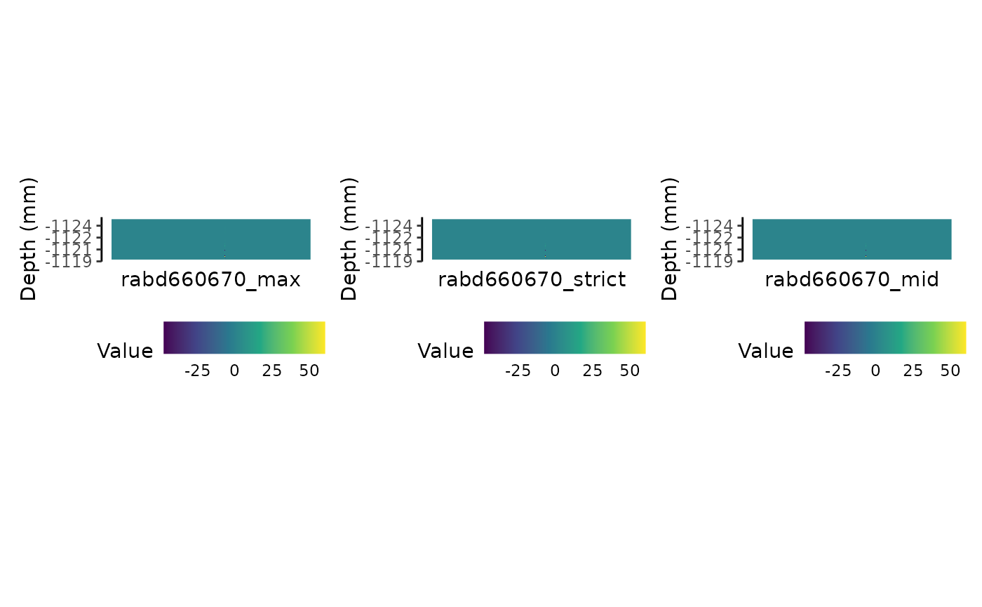

Similar, but not identical. As expected!

Relative Absorption Band Area (RABA)

Band ratios

Another popular and straightforward index is band ratios, where reflectance at wavelength X is divided by reflectance at wavelength Y.

ratio_570630 <- reflectance_smooth |>
  calculate_band_ratio(
    edges = proxies$ratio_b570b630$edges,
    ratio_name = proxies$ratio_b570b630$proxy_name)

plot_ratio570630 <- ratio_570630 |>
  plot_raster_proxy(
    hsi_index = names(ratio_570630),
    palette = "magma",
    calibration = pixel_to_distance(core))

plot_ratio570630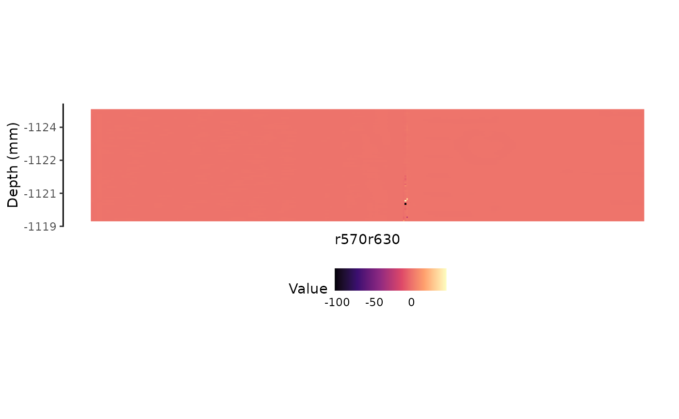

Band differences

difference_650675 <- reflectance_smooth |>
  calculate_band_difference(
    difference_name = proxies$diff_b650b675$proxy_name,
    edges = proxies$diff_b650b675$edges)

plot_difference_650675 <- difference_650675 |>
  plot_raster_proxy(
    hsi_index = names(difference_650675),
    palette = "cividis",
    calibration = pixel_to_distance(core))

plot_difference_650675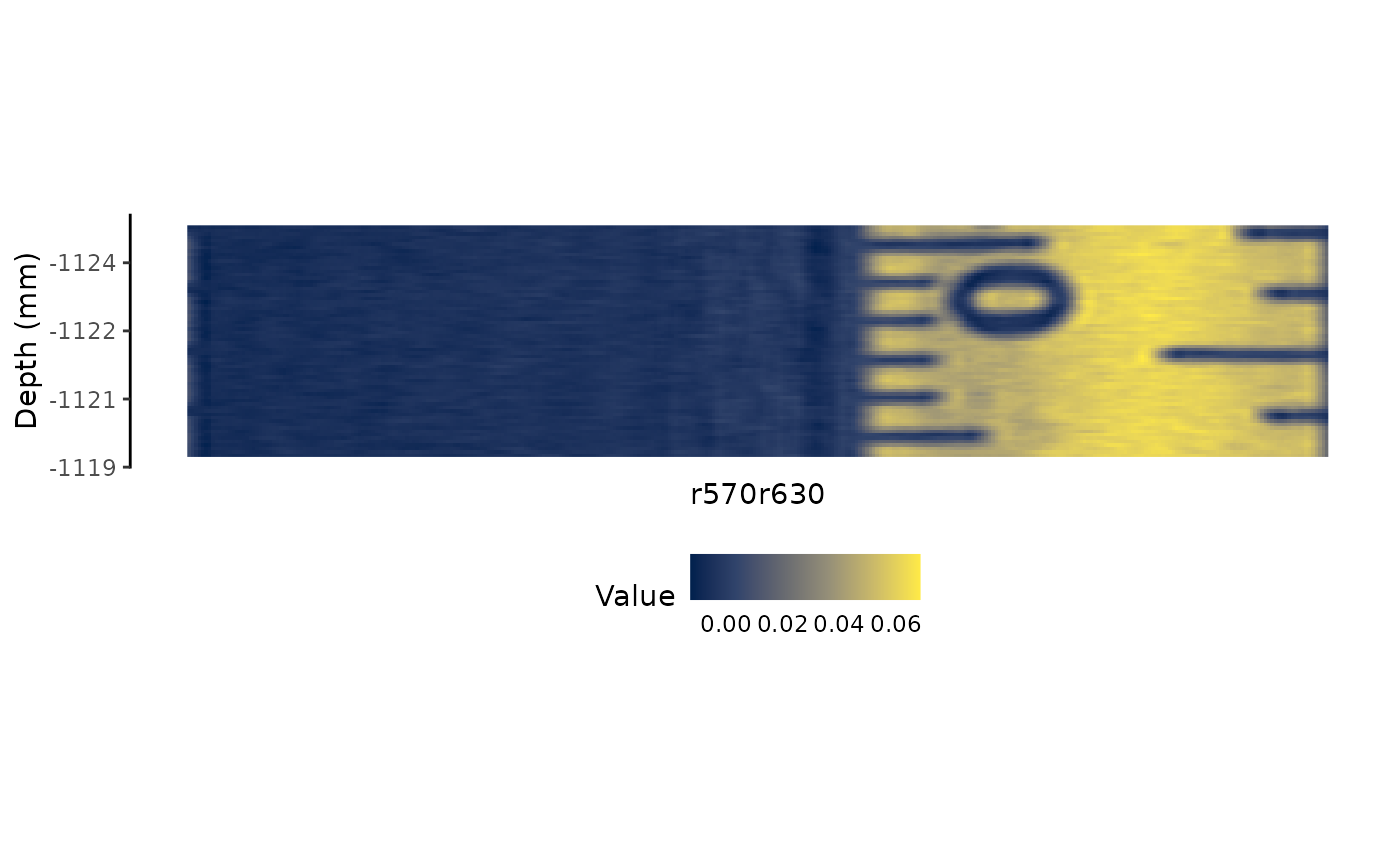

Derivatives

# derivative_690 <- reflectance_smooth |>
#   calculate_derivative(derivative_name = proxies$deriv_b690)

lambdaREMP

This index was introduced in the paper “Ghanbari, H., Zilkey, D.R., Gregory-Eaves, I., Antoniades, D., 2023. A new index for the rapid generation of chlorophyll time series from hyperspectral imaging of sediment cores. Limnology and Oceanography: Methods 21, 703–717. https://doi.org/10.1002/lom3.10576”

# lambdaremp <- reflectance_smooth |>
#   calculate_remp()

Savitzky, Abraham., and M. J. E. Golay. 1964. “Smoothing and Differentiation of Data by Simplified Least Squares Procedures.” Analytical Chemistry 36 (8): 1627–39. https://doi.org/10.1021/ac60214a047.