Spectral indices catalogue
HSItools includes a built-in catalogue of spectral indices drawn from the literature. It is a practical starting point for common sediment proxies, not a comprehensive literature review.
# Show tibble
HSItools::spectral_indices
#>        proxy_name proxy_type continuum_edges absorption_band index_type
#> 1         rabd510       rabd        590, 730             510     strict
#> 2         rabd615       rabd        590, 730             615     strict
#> 3  rabd615_narrow       rabd        590, 640             615     strict
#> 4      rabd640655       rabd        590, 730        640, 655        max
#> 5         rabd660       rabd        590, 730             660     strict
#> 6      rabd660670       rabd        590, 730        660, 670        max
#> 7         rabd845       rabd        790, 900             845     strict
#> 8    rabd16601690       rabd              NA              NA       <NA>
#> 9      raba650700       raba        650, 700              NA          x
#> 10     raba600760       raba        600, 760              NA          x
#> 11     raba590730       raba        590, 730              NA          x
#> 12     raba650750       raba        650, 750              NA          x
#> 13    ratio570630      ratio              NA              NA       <NA>
#> 14    ratio590690      ratio              NA              NA       <NA>
#> 15    ratio590640      ratio              NA              NA       <NA>
#> 16    ratio645675      ratio              NA              NA       <NA>
#> 17    ratio660670      ratio              NA              NA       <NA>
#> 18    ratio675750      ratio              NA              NA       <NA>
#> 19    ratio650675      ratio              NA              NA       <NA>
#> 20    ratio850900      ratio              NA              NA       <NA>
#> 21    ratio950970      ratio              NA              NA       <NA>
#> 22     diff675750 difference              NA              NA       <NA>
#> 23     diff650675 difference              NA              NA       <NA>
#> 24     diff660690 difference              NA              NA       <NA>
#> 25           remp       remp              NA              NA       <NA>
#>       bands search_range                              interpretation
#> 1        NA           NA                                 carotenoids
#> 2        NA           NA                                 phycocyanin
#> 3        NA           NA                                      albite
#> 4        NA           NA                         total chlorophyll-a
#> 5        NA           NA                         total chlorophyll-a
#> 6        NA           NA                         total chlorophyll-a
#> 7        NA           NA                       bacteriophaeophytin-a
#> 8        NA           NA                 terrestrial aromatic matter
#> 9        NA           NA                         total chlorophyll-a
#> 10       NA           NA                         total chlorophyll-a
#> 11       NA           NA                         total chlorophyll-a
#> 12       NA           NA                         total chlorophyll-a
#> 13 570, 630           NA                         clay minerals, dust
#> 14 590, 690           NA                         clay minerals, dust
#> 15 590, 640           NA lithogenic content (illite, chlorite, mica)
#> 16 645, 675           NA                         clay minerals, dust
#> 17 660, 670           NA           degree of photopigment diagenesis
#> 18 675, 750           NA                         clay minerals, dust
#> 19 650, 675           NA                         clay minerals, dust
#> 20 850, 900           NA                         clay minerals, dust
#> 21 950, 970           NA                         clay minerals, dust
#> 22 675, 750           NA                         clay minerals, dust
#> 23 650, 675           NA                         clay minerals, dust
#> 24 660, 690           NA                         clay minerals, dust
#> 25       NA           NA                         total chlorophyll-a
#>                                                             reference
#> 1                                                                <NA>
#> 2                                                                <NA>
#> 3  von Gunten et al. (2012) https://doi.org/10.1007/s10933-012-9582-9
#> 4                                                                <NA>
#> 5                                                                <NA>
#> 6                                                                <NA>
#> 7                                                                <NA>
#> 8                                                                <NA>
#> 9                                                                <NA>
#> 10                                                               <NA>
#> 11                                                               <NA>
#> 12                                                               <NA>
#> 13                                                               <NA>
#> 14                                                               <NA>
#> 15 von Gunten et al. (2012) https://doi.org/10.1007/s10933-012-9582-9
#> 16                                                               <NA>
#> 17 von Gunten et al. (2012) https://doi.org/10.1007/s10933-012-9582-9
#> 18                                                               <NA>
#> 19                                                               <NA>
#> 20                                                               <NA>
#> 21                                                               <NA>
#> 22                                                               <NA>
#> 23                                                               <NA>
#> 24                                                               <NA>
#> 25          Ghanbari et al. (2023) https://doi.org/10.1002/lom3.10576
You can filter by proxy_type to see what is available for a given calculation method:
HSItools::spectral_indices |>
  dplyr::filter(proxy_type == "rabd")
#> # A tibble: 8 × 9
#>   proxy_name     proxy_type continuum_edges absorption_band index_type bands
#>   <chr>          <chr>      <list>          <list>          <chr>      <list>
#> 1 rabd510        rabd       <dbl [2]>       <dbl [1]>       strict     <lgl [1]>
#> 2 rabd615        rabd       <dbl [2]>       <dbl [1]>       strict     <lgl [1]>
#> 3 rabd615_narrow rabd       <dbl [2]>       <dbl [1]>       strict     <lgl [1]>
#> 4 rabd640655     rabd       <dbl [2]>       <dbl [2]>       max        <lgl [1]>
#> 5 rabd660        rabd       <dbl [2]>       <dbl [1]>       strict     <lgl [1]>
#> 6 rabd660670     rabd       <dbl [2]>       <dbl [2]>       max        <lgl [1]>
#> 7 rabd845        rabd       <dbl [2]>       <dbl [1]>       strict     <lgl [1]>
#> 8 rabd16601690   rabd       <lgl [1]>       <lgl [1]>       <NA>       <lgl [1]>
#> # ℹ 3 more variables: search_range <list>, interpretation <chr>,
#> #   reference <chr>
Calculating spectral indices
Given the known spectral features, we can now calculate our first spectral index of choice. To calculate an index, pass the spectral parameters directly to the corresponding function. We are going to use test reflectance previously processed with hsi_smooth_median() and hsi_smooth_savgol(). We also need a derivative raster.
r <- terra::rast(
  system.file(
    package = "HSItools",
    "testdata/products/SAVGOL_testdata.tif"
  )
)
Relative Absorption Band Depth
Relative Absorption Band Depth (RABD) is a straightforward type of index, often used for sediment scanning data. Calculate RABD centered around 660 nm to see relative chlorophyll-a abundance.
# A "strict" variant pointing at a given wavelength
rabd660 <- HSItools::hsi_calc_rabd(
  r,
  continuum_edges = c(590, 730),
  absorption_band = 660,
  index_type = "strict",
  index_name = "rabd660",
  filename = tempfile(fileext = ".tif"),
  overwrite = TRUE
)

rabd660
#> class       : SpatRaster
#> size        : 9, 9, 1  (nrow, ncol, nlyr)
#> resolution  : 1, 1  (x, y)
#> extent      : 1000, 1009, 2000, 2009  (xmin, xmax, ymin, ymax)
#> coord. ref. :
#> source(s)   : memory
#> varname     : SAVGOL_testdata
#> name        :  rabd660
#> min value   : 1.002019
#> max value   : 1.043918
# A "max" variant flexibly selecting wavelength of a minimum reflectance value in a range
rabd660670 <- HSItools::hsi_calc_rabd(
  r,
  continuum_edges = c(590, 730),
  absorption_band = c(660, 670),
  index_type = "max",
  index_name = "rabd660670",
  filename = tempfile(fileext = ".tif"),
  overwrite = TRUE
)

rabd660670
#> class       : SpatRaster
#> size        : 9, 9, 1  (nrow, ncol, nlyr)
#> resolution  : 1, 1  (x, y)
#> extent      : 1000, 1009, 2000, 2009  (xmin, xmax, ymin, ymax)
#> coord. ref. :
#> source(s)   : memory
#> varname     : SAVGOL_testdata
#> name        : rabd660670
#> min value   :   1.002019
#> max value   :   1.043918
Band Ratio
Band ratio is a simple index where reflectance at band A is divided by reflectance at band B.
ratio660670 <- HSItools::hsi_calc_ratio(
  r,
  bands = c(660, 670),
  index_name = "ratio660670",
  filename = tempfile(fileext = ".tif"),
  overwrite = TRUE
)

ratio660670
#> class       : SpatRaster
#> size        : 9, 9, 1  (nrow, ncol, nlyr)
#> resolution  : 1, 1  (x, y)
#> extent      : 1000, 1009, 2000, 2009  (xmin, xmax, ymin, ymax)
#> coord. ref. :
#> source(s)   : memory
#> varname     : SAVGOL_testdata
#> name        : ratio660670
#> min value   :    0.984696
#> max value   :    1.002303
Band Difference
Band difference subtracts reflectance at band B from reflectance at band A.
diff660690 <- HSItools::hsi_calc_difference(
  r,
  bands = c(660, 690),
  index_name = "diff660690",
  filename = tempfile(fileext = ".tif"),
  overwrite = TRUE
)

diff660690
#> class       : SpatRaster
#> size        : 9, 9, 1  (nrow, ncol, nlyr)
#> resolution  : 1, 1  (x, y)
#> extent      : 1000, 1009, 2000, 2009  (xmin, xmax, ymin, ymax)
#> coord. ref. :
#> source(s)   : memory
#> varname     : SAVGOL_testdata
#> name        : diff660690
#> min value   :  -0.022675
#> max value   :  -0.009948
Red-Edge Minimum Point
λREMP is an index meant for chlorophyll-a detection proposed by Ghanbari et al. (2023). It uses the first derivative of the spectrum to find exact wavelength where the absorbance near the red edge reaches minimum (zero crossing in derivative space). The wavelength (nm) is the index value. By default we are looking for minimum value (dip) in 660 nm to 680 nm.
remp <- terra::rast(
  system.file(
    package = "HSItools",
    "testdata/products/MEDIAN_testdata.tif"
  )
) |>
  # Calculate 1st derivative
  HSItools::hsi_smooth_savgol(m = 1) |>
  # Calculate REMP
  HSItools::hsi_calc_remp(
    search_range = c(660, 680),
    filename = tempfile(fileext = ".tif"),
    index_name = "remp",
    overwrite = TRUE
  )

remp
#> class       : SpatRaster
#> size        : 9, 9, 1  (nrow, ncol, nlyr)
#> resolution  : 1, 1  (x, y)
#> extent      : 1000, 1009, 2000, 2009  (xmin, xmax, ymin, ymax)
#> coord. ref. :
#> source      : file22af4577b22d.tif
#> name        :       remp
#> min value   : 661.280029
#> max value   : 666.400024
Using the catalogue
Instead of typing spectral parameters manually, you can look them up directly from spectral_indices and pass them to the function. This is useful when running multiple indices or when you want to keep your code tied to a single source of truth. Here we recalculate rabd660670 using the catalogue rather than typed parameters. The result is identical.
# Pull the rabd660670 entry
idx <- HSItools::spectral_indices |>
  dplyr::filter(proxy_name == "rabd660670")

# Pass parameters to the function
rabd660670 <- HSItools::hsi_calc_rabd(
  x = r,
  continuum_edges = idx$continuum_edges[[1]],
  absorption_band = idx$absorption_band[[1]],
  index_type = idx$index_type,
  index_name = "rabd660670",
  filename = tempfile(fileext = ".tif"),
  overwrite = TRUE
)

rabd660670
#> class       : SpatRaster
#> size        : 9, 9, 1  (nrow, ncol, nlyr)
#> resolution  : 1, 1  (x, y)
#> extent      : 1000, 1009, 2000, 2009  (xmin, xmax, ymin, ymax)
#> coord. ref. :
#> source(s)   : memory
#> varname     : SAVGOL_testdata
#> name        : rabd660670
#> min value   :   1.002019
#> max value   :   1.043918
Data extraction
Extract index profile
Spatial data is an important foundation of HSI, however, at the end we are often interested in getting a single profile representing an index.
rabd_profile <- rabd660670 |>
  HSItools::hsi_extract_profile()

rabd_profile
#> # A tibble: 9 × 2
#>   position rabd660670
#>      <dbl>      <dbl>
#> 1    2008.       1.02
#> 2    2008.       1.03
#> 3    2006.       1.02
#> 4    2006.       1.03
#> 5    2004.       1.02
#> 6    2004.       1.03
#> 7    2002.       1.02
#> 8    2002.       1.01
#> 9    2000.       1.02
You can also easilly plot these values with a helper function. These are ggplot2 objects that can be easily modified with +. Please mind, that at this moment we are using the terra pixel space. Spatial calibration is covered in spatial calibration vignette.
The plot function requires the index raster to have a named layer. Pass
index_namewhen calculating to ensure this..
rabd_profile |> HSItools::hsi_plot_profile()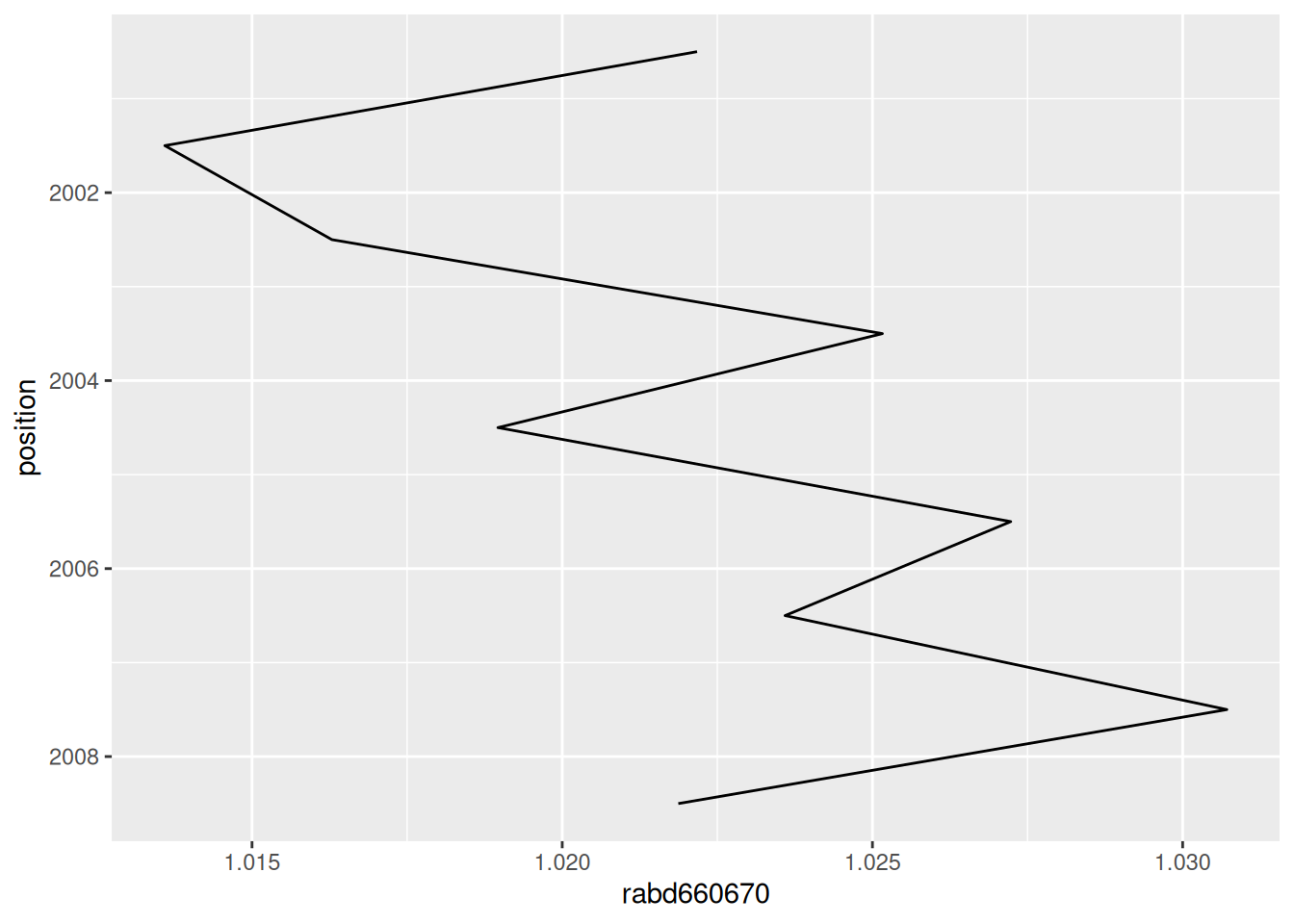
Extract reflectance profile
Reflectance profile in a region of choice is a good diagnostic tool. It can be easilly pulled.
r_profile <- r |>
  HSItools::hsi_extract_spectrum()

r_profile
#> # A tibble: 101 × 2
#>    wavelength value
#>         <dbl> <dbl>
#>  1       518. 0.149
#>  2       520. 0.151
#>  3       523. 0.154
#>  4       525. 0.157
#>  5       528. 0.160
#>  6       530. 0.162
#>  7       532. 0.165
#>  8       535. 0.167
#>  9       537. 0.170
#> 10       540. 0.172
#> # ℹ 91 more rows
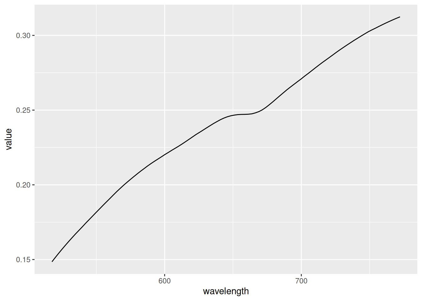
You can also easilly plot these values with a helper function, just like the hsi_extract_profile() output.
r_profile |> HSItools::hsi_plot_spectrum()